Predicting user churn
- Apr 3, 2023
- 6 min read
Problem Statement

An X Education need help to select the most promising leads, i.e. the leads that are most likely to convert into paying customers. The company requires us to build a model wherein you need to assign a lead score to each of the leads such that the customers with higher lead score have a higher conversion chance and the customers with lower lead score have a lower conversion chance.
Aim
To build a logistic regression model to assign a lead score between 0 and 1 to each of the leads which can be used by the company to target potential leads. A higher score would mean that the lead is hot, i.e. is most likely to convert whereas a lower score would mean that the lead is cold and will mostly not get converted.
Dataset
The dataset has 37 columns and 9240 rows.
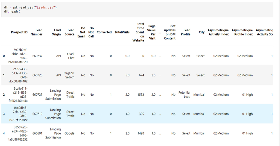
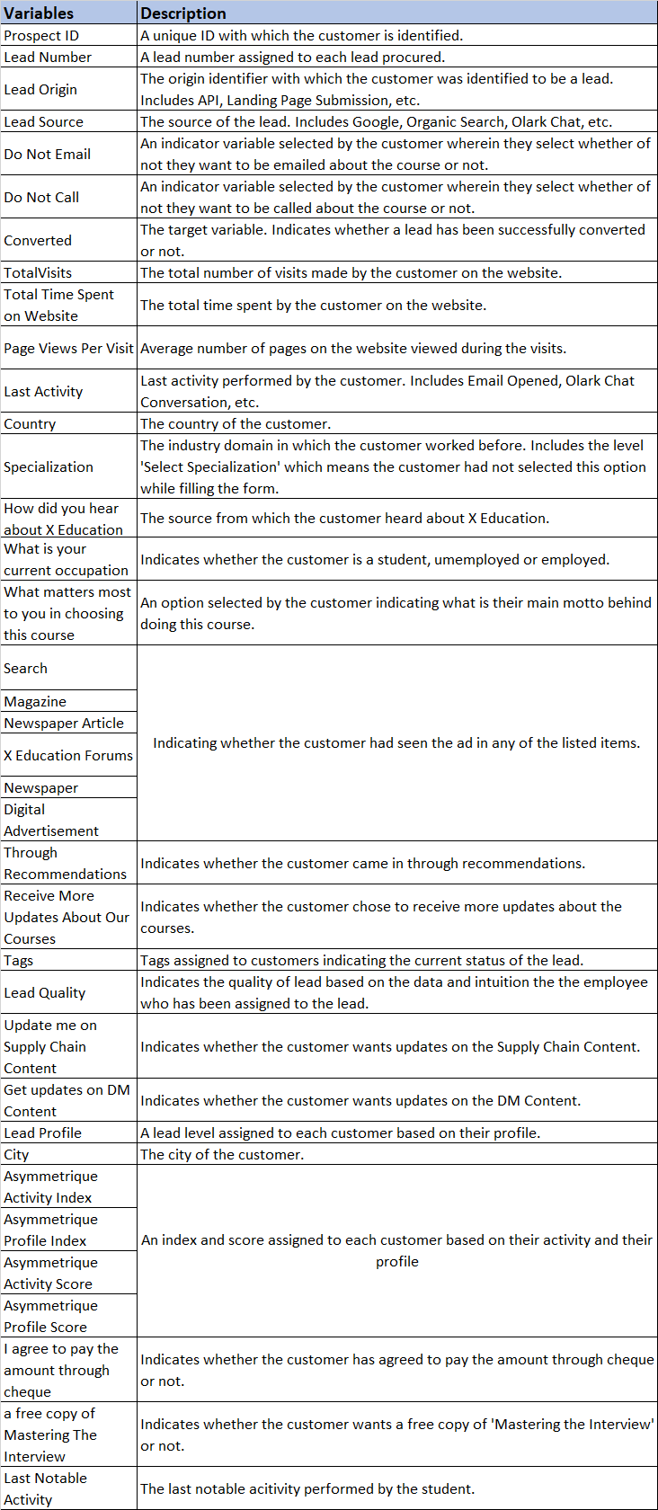
The dataset has numerical and categorical columns. The below table explains each column:
Data Cleaning
The dataset has several unwanted columns that have no impact on the user's purchase like purchasing a 'free copy of mastering the interview', 'update me on supply chain content' and more and hence these variables are dropped. Also, several variables that have more than 35% null values are dropped
# Removing all the columns that are not required and have 35% null values

df = df.drop(['Asymmetrique Profile Index','Asymmetrique Activity Index','Asymmetrique Activity Score','Asymmetrique Profile Score','Lead Profile','Tags','Lead Quality','How did you hear about X Education','City','Lead Number'],axis=1)

# Dropping unique valued columns
df= df.drop(['Magazine','Receive More Updates About Our Courses','I agree to pay the amount through cheque','Get updates on DM Content','Update me on Supply Chain Content'],axis=1)
Certain values that can not be dropped despite having null values since they are useful to build the model. We replace them with most frequent choices or NAN
df = df.replace('select',np.nan)df['Specialization'] = df['Specialization'].fillna('not provided')
df['What matters most to you in choosing a course'] = df['What matters most to you in choosing a course'].fillna('not provided')
df['Country'] = df['Country'].fillna('not provided')
df['What is your current occupation'] = df['What is your current occupation'].fillna('not provided')
df.info()Exploring the dataset
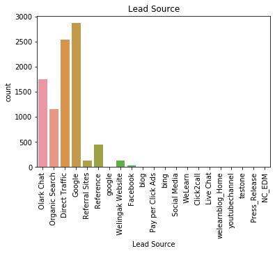
Most of the users are directed to the website from google, direct search or organic traffic. Other websites that the company has been promoted on does not seem to work.
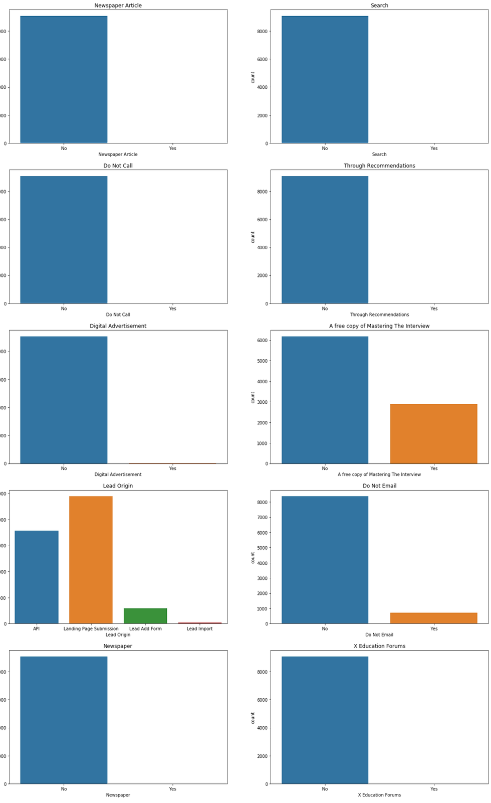
The above plots show the preferred choices of customers and what they opt on the website.
Inspecting continuous data
The below charts describe the most important continuous dataset that is important to predict churn rate.
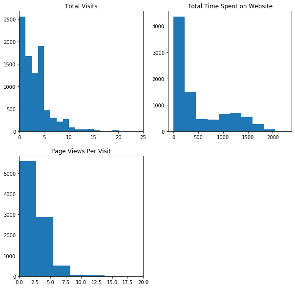
Most people spend abut 250-300 seconds on the website (around 4-5 minutes)
On an average, people visit 2.5 pages and re-visit the website on an average of 2 times
Re-checking variables
Although a lot of variables seem like they contribute to the churn rate but need not. This can only be understood by observing the relationship between certain variables and whether they churned or not.
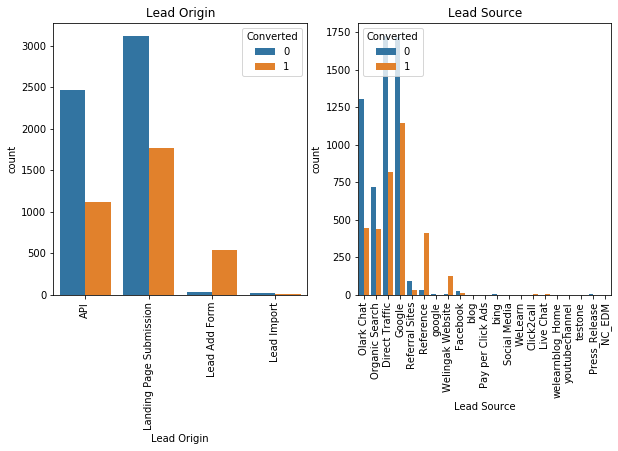
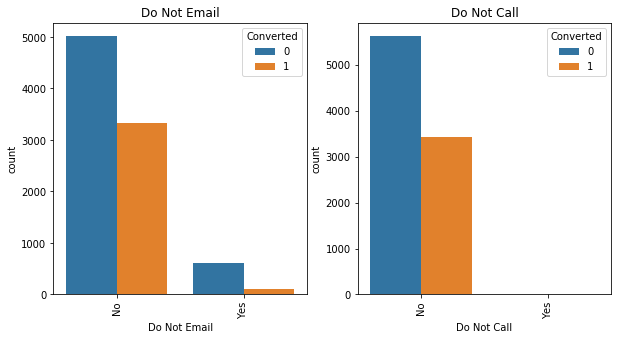

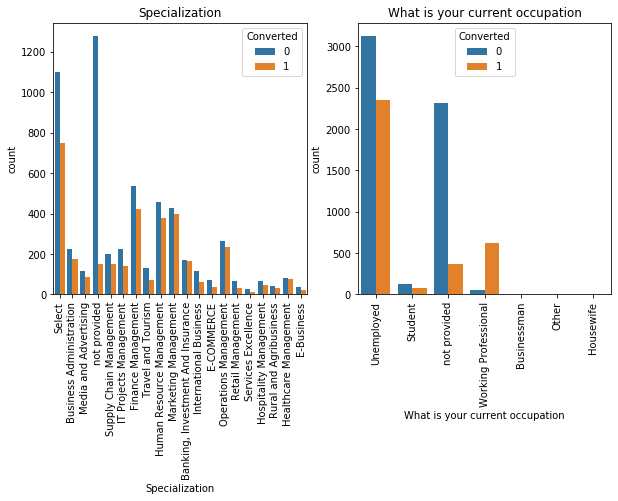
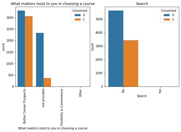
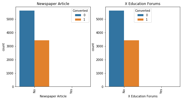
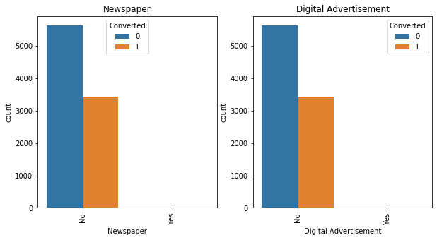
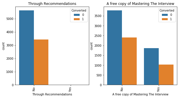
We drop certain variables that don't seem to have an impact on the variables. Before that we create important dummy variables for those that are important and contribute to the churn rate
# Creating dummy variables using the 'get_dummies'
dummy = pd.get_dummies(df[['Lead Origin','Specialization' ,'Lead Source', 'Do Not Email', 'Last Activity', 'What is your current occupation','A free copy of Mastering The Interview', 'Last Notable Activity']], drop_first=True)

# Adding the results to the master dataframe
df = pd.concat([df, dummy], axis=1)
Dropping variables that are not important any more:
df = df.drop(['What is your current occupation_not provided','Lead Origin', 'Lead Source', 'Do Not Email', 'Do Not Call','Last Activity', 'Country', 'Specialization', 'Specialization_not provided','What is your current occupation','What matters most to you in choosing a course', 'Search','Newspaper Article', 'X Education Forums', 'Newspaper','Digital Advertisement', 'Through Recommendations','A free copy of Mastering The Interview', 'Last Notable Activity'], axis=1)These variables vary with the churn rate and hence are dropped
Building the model
First we split the dataset to test and train so that we can be sure the model is consistent for all kinds of values.
from sklearn.model_selection import train_test_splitThen we split the data into independent and dependent variables
X = df.drop(['Converted'], 1)
y = df['Converted']
The data is split in test and train in the ratio of 7:3
X_train, X_test, y_train, y_test = train_test_split(X, y, train_size=0.7, test_size=0.3, random_state=10)
Scaling
There are several variables that are in different units of measurement. This can impact the accuracy of the prediction and hence we normalize it to make all values range between 0 and 1
from sklearn.preprocessing import MinMaxScaler
# Scale the three numeric features
scaler = MinMaxScaler()
X_train[['TotalVisits', 'Page Views Per Visit', 'Total Time Spent on Website']] = scaler.fit_transform(X_train[['TotalVisits', 'Page Views Per Visit', 'Total Time Spent on Website']])
X_train.head()
Finding the most important variables
To find the most important variables, we use feature selection from the sci-kit learn library
from sklearn.feature_selection import RFE
rfe = RFE(logreg, 15)
rfe = rfe.fit(X_train, y_train)
list(zip(X_train.columns, rfe.support_, rfe.ranking_))
col = X_train.columns[rfe.support_]
X_train = X_train[col]
Fitting the model
# Importing statsmodels
import statsmodels.api as sm

X_train_sm = sm.add_constant(X_train)
logm1 = sm.GLM(y_train, X_train_sm, family = sm.families.Binomial())
res = logm1.fit()
res.summary()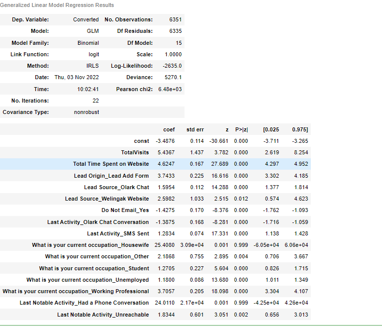
With most variables showing significance, we can say the model is a good predictor but there could also be some over-fitting as well. Also, a few variables are insignificant and hence need to be removed or re-checked in the new model
Multicollinearity check
from statsmodels.stats.outliers_influence import variance_inflation_factorvif = pd.DataFrame()
vif['Features'] = X_train.columns
vif['VIF'] = [variance_inflation_factor(X_train.values, i) for i in range(X_train.shape[1])]
vif['VIF'] = round(vif['VIF'], 2)
vif = vif.sort_values(by = "VIF", ascending = False)
vif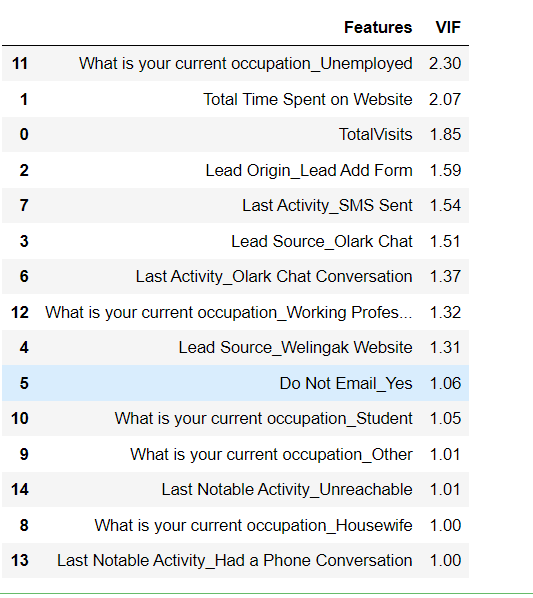
There is no multicollinearity as VIF is below 5 which shows that there is very low correlation or no correlation between the variables. The variables are a good predictor and despite some variables having low significance, it is important to keep them for this particular business case as these are important variables that predict a purchase of the online course.
Making the prediction
y_train_pred = res.predict(X_train_sm)
y_train_pred[:10]

# Substituting 0 or 1 with the cut off as 0.5

y_train_pred_final['Predicted'] = y_train_pred_final.Conversion_Prob.map(lambda x: 1 if x > 0.5 else 0)
y_train_pred_final.head()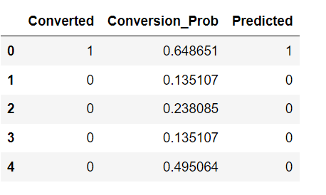
Evaluating the model
Checking accuracy
from sklearn import metrics
metrics.accuracy_score(y_train_pred_final.Converted, y_train_pred_final.Predicted)0.810266099826799We can observe that it has 81% accuracy.
We build a confusion matrix to check specificity and sensitivity
confusion = metrics.confusion_matrix(y_train_pred_final.Converted, y_train_pred_final.Predicted )
confusion
Calculating Positive and Negative variants
# Substituting the value of true positive
TP = confusion[1,1]
# Substituting the value of true negatives
TN = confusion[0,0]
# Substituting the value of false positives
FP = confusion[0,1]
# Substituting the value of false negatives
FN = confusion[1,0]
Specificity:
TP/(TP+FN)0.6954397394136808Sensitivity:
TN/(TN+FP)0.8826700898587934Despite having a high accuracy and sensitivity, it is important to have high specificity since these are the customers that can potentially become purchasing users and hence we need to have a high specificity ensuring high accuracy and sensitivity as well.
Making ROC curve
We check our ROC curve to see how good the model predicts. Essentially the true positive rate should be high and the false positive rate should be low.
# ROC function
def draw_roc( actual, probs ):
    fpr, tpr, thresholds = metrics.roc_curve( actual, probs,
                                              drop_intermediate = False )
    auc_score = metrics.roc_auc_score( actual, probs )
    plt.figure(figsize=(5, 5))
    plt.plot( fpr, tpr, label='ROC curve (area = %0.2f)' % auc_score )
    plt.plot([0, 1], [0, 1], 'k--')
    plt.xlim([0.0, 1.0])
    plt.ylim([0.0, 1.05])
    plt.xlabel('False Positive Rate or [1 - True Negative Rate]')
    plt.ylabel('True Positive Rate')
    plt.title('Receiver operating characteristic example')
    plt.legend(loc="lower right")
    plt.show()

    return None
fpr, tpr, thresholds = metrics.roc_curve( y_train_pred_final.Converted, y_train_pred_final.Conversion_Prob, drop_intermediate = False )# Call the ROC function
draw_roc(y_train_pred_final.Converted, y_train_pred_final.Conversion_Prob)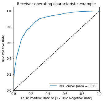
The larger the area under the curve tells us that it is a good model. Since the area under the curve is 88% of the total area, it is safe to say that the model is significant. Now, to optimize the model we can check for better cutoff rates than 0.5
Evacuating probability cutoff value
Creating columns with different probability cutoffs:
numbers = [float(x)/10 for x in range(10)]
for i in numbers:
    y_train_pred_final[i]= y_train_pred_final.Conversion_Prob.map(lambda x: 1 if x > i else 0)
y_train_pred_final.head()
# Creating a dataframe to see the values of accuracy, sensitivity, and specificity at different values of probabiity cutoffs
cutoff_df = pd.DataFrame( columns = ['prob','accuracy','sensi','speci'])

# Making confusing matrix to find values of sensitivity, accurace and specificity for each level of probablity

from sklearn.metrics import confusion_matrix
num = [0.0,0.1,0.2,0.3,0.4,0.5,0.6,0.7,0.8,0.9]

for i in num:
    cm1 = metrics.confusion_matrix(y_train_pred_final.Converted, y_train_pred_final[i] )
    total1=sum(sum(cm1))
    accuracy = (cm1[0,0]+cm1[1,1])/total1

    speci = cm1[0,0]/(cm1[0,0]+cm1[0,1])
    sensi = cm1[1,1]/(cm1[1,0]+cm1[1,1])
    cutoff_df.loc[i] =[ i ,accuracy,sensi,speci]
   cutoff_df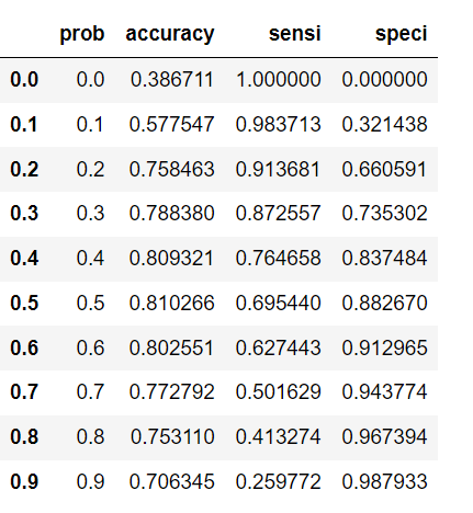
We can observe the accuracy, specificity and the sensitivity for different probability cutoff rates.
cutoff_df.plot.line(x='prob', y=['accuracy','sensi','speci'])
plt.show()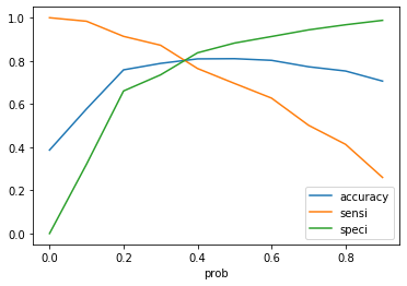
It can be observed that the point near 0.35 is the ideal probability cutoff where the tradeoff between accuracy, specificity and sensitivity is the lowest.
Re-building the model
The model is re-built with 0.35 as the cutoff rate.
y_train_pred_final['final_predicted'] = y_train_pred_final.Conversion_Prob.map( lambda x: 1 if x > 0.35 else 0)
y_train_pred_final.head()
Checking accuracy, specificity and sensitivity
Accuracy is calculated using inbuilt function:
metrics.accuracy_score(y_pred_final['Converted'], y_pred_final.final_predicted)0.80940139551964confusion2 = metrics.confusion_matrix(y_pred_final['Converted'], y_pred_final.final_predicted )Calculating the positive and negative variants
# Substituting the value of true positive
TP = confusion2[1,1]
# Substituting the value of true negatives
TN = confusion2[0,0]
# Substituting the value of false positives
FP = confusion2[0,1]
# Substituting the value of false negatives
FN = confusion2[1,0]
# Calculating the specificity
TP/(TP+FN)0.81511746680286# Calculating the sensitivity
TN/(TN+FP)0.8061926605504587We can observe that the accuracy is still around the same amount and the sensitivity and specificity have also increased which makes this the best model.
Conclusion
The model is built to predict the churn rate to provide discounts and offers to most potential customers that can be converted into purchasing users. The model predicts the churn probability with an accuracy of 81%.
The model also has a high specificity which is very important for this particular instance as it is important to not lose out on warm and hot leads
It also has a high sensitivity which is useful as offers and discounts need not be spent on customers that were most likely not going to buy in the first place which reduces expenses.


Comments